|
BIOMCON Infoletter 2013/#1 |
Bio-Math-Consulting |
||
|
|
|
||
|
|
|||
|
Population Evolution Charts? What’s that? By Dr. Joachim Moecks, BIOMCON GmbH, Mannheim, Germany March 2013 |
|
||

|
Introduction: In many clinical studies the clinical endpoints are of the type time-to-progression, time to worsening, time to relapse etc, i.e. time-to-event data. The idea underlying the Population Evolution Charts (PEC) for these data is simple:
Suppose the study starts at baseline with 70 % males and 30% females. What would you say if after some study time the percentage of males in the cohort at risk decreased to approx. 50%?
Certainly one would conclude that the events selected predominantly males out of the baseline cohort. Actually, if the probability for an event occurring in a male rather than female were about 0.7, we would not see any decline in the percentage of males, since we started out with 70% of males. Thus this probability must be definitely higher than 0.7 – in other words, there seems to be some association between gender and the occurrence of events.
The PEC here is simply defined by monitoring the percentage of males in the patient cohort (at risk) over treatment time. It should be clear, that we may replace gender by any other (binary) baseline covariate, e.g. young vs. old, or by a special baseline diagnose group. Here is to emphasize, that PECs do not deal with time varying covariates – only baseline covariates are considered. The time-varying feature of a PEC is the time-varying composition of the cohort at risk with respect to these baseline variables. Here see the basic scheme of interpretation:
|
|||||||||||||||
|
|
|||||||||||||||
|
In which data is the analysis by PECs useful? Whenever the study is big an enough that you would consider Kaplan-Meier curves then PECs can be an easy way to study the relation between the events and interesting covariates.
And even more –
Real data examples illustrate these points:
|
|||||||||||||||
|
|
|||||||||||||||
|
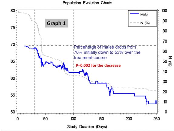
The first example (graph1) features the decline of percentage of males during the study. We may accept that this is a steady decrease and therefore a Cox-regression to find the hazard ratio between male and females could be a next step.
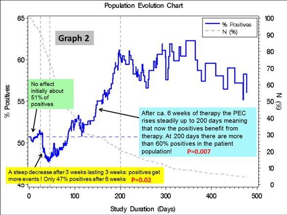
The second graph shows a more complicated pattern. The PEC here features the percentage of biomarker positives over time. After a steep decrease - indicating that positives had more events - the PEC rises again meaning then that positives had fewer events. The application of Cox regression cannot be recommended here, since the assumption of proportional hazards is grossly violated.
|
|||||||||||||||
|
|
|||||||||||||||
|
A little more mathematical detail: The classical approach to time-to-event data focuses on estimation of survivor functions and related statistical tests. When the association to covariates is to be studied, then the gold standard is use of Cox’ proportional hazard model.
Population evolution charts (PEC) address covariates from a different angle by considering the development of the cohort over time as a selection process: if the covariate is not associated with the events, one does not expect a change in distribution of the covariates over time – i.e. the covariate is indifferent with respect to the event process. If the covariate is selective (i.e. influences the probability of an event), then a change in distribution over time can be expected. In short, while the usual regression approach is modelling P(T > t | X = x), the PEC looks at it reversely P(X = x | T > t).
Population evolution charts need only few assumptions. They originated in purely descriptive approaches [1]. In particular the time dynamic of the hazard ratio development can be readily observed, which provides in many cases additional insights for the event process. The time pattern of effects can reveal important interactions in controlled designs [2].
The mathematical analysis of the PEC approach for binary covariates can be found in [3] (download below). It includes a discussion of the relation of PECs and Cox-regression, necessary conditions for the validity of proportional hazards, and includes an example how to achieve explicit estimates of the hazard functions.
After these basic facts, statistical tests were developed to address different aspects of the PEC course. The hypothesis of global PEC constancy can be tested in principle by the log-rank test (see [3]) – however, for non-monotonic PEC’s this test shows no power. To this end, we used Wald-Wolfowitz runs test. For local hypotheses as in graph2, we employed calculations based on the hypergeometric distribution. These alternative testing options were reported in a talk at the University of Heidelberg in November 2012 (download below). Here we report the test results pertaining to graph1 and 2.
PEC’s can be defined for metric baseline covariates. Then characteristics of the distribution of the covariate in the cohort at risk are studied over study time – e.g. moments, quantiles etc. These extensions were also discussed in the Heidelberg talk.
References
[1] Moecks J., Franke W., Ehmer B., Quarder O. (1997): Analysis of Safety Database for Long-Term Epoetin-β Treatment: A Meta-Analysis Covering 3697 Patients. In: Koch & Stein (editors) “Pathogenetic and Therapeutic Aspects of Chronic Renal Failure”. Marcel Dekker: New York, 163-179.
[2] Moecks J., Köhler W., Scott M., Maurer J., Budde M., Givens S.(2002): Dealing with Selective Dropout in Clinical Trials. Pharmaceutical Statistics, Vol 1: 119-130
[3] Moecks J., Koehler W.(2007): Population Evolution Charts: A Fresh Look to Time-To-Event Data. Statistical Computing and Graphics, Vol. 18, No 2, Dec 2007, p. 12-19
|
|||||||||||||||
|
|
|||||||||||||||
|

|
bioMcon GmbH | Max-Joseph-Str. 9 | D-68167 Mannheim | Tel. +49 (0) 621/1287361 | Email:info@biomcon.com |